This model is featured because its Hugging Face README.md includes an hfviewer architecture visualization.
Interactive model architecture
Architecture graph for embedl/Qwen3-1.7B-FlashHead-W4A16.
Interactive architecture graph for embedl/Qwen3-1.7B-FlashHead-W4A16, visualized from Hugging Face model metadata.
Paste a Hugging Face link to visualize it
No export step, no config hunt, no model surgery. Paste the link and inspect the graph.
Graph structure
Understand the high-level graph structure of different transformer models.
Quickstart guide
URL magic
You can replace huggingface.co with hfviewer.com in the url to view it.